Introduction
If you don’t want to listen to our long-winded theory, please move to the Quick start

Snapshot description
MCnebula2 was used for metabonomics data analysis. It is written in the S4
system of object-oriented programming, starts with and also ends with a
“class”, namely mcnebula. The whole process takes the mcnebula as the
operating object to obtain visual results or operating objects.
Most methods of MCnebula2 are S4 methods and have the characteristics of
parameterized polymorphism, that is, different functions will be used for
processing according to different parameters passed to the same method; use
empty parameter with Methods may return the default parameters for the methods
(such as cross_filter_stardust()).
MCnebula workflow is a complete metabolomics data analysis process, including initial data preprocessing (data format conversion, feature detection), compound identification based on MS/MS, statistical analysis, focusing of compound structure and chemical class, multi-level data visualization, output report, etc.
It should be noted that the MCnebula2 R package currently cannot realize the entire analysis process of MCnebula workflow. If users want to complete the entire workflow, other software beyond the R console (for example, the MSconvert tool of proteowizard is used for data format conversion; SIRIUS is used for computational prediction of compounds) should be used. This is a pity, but we will gradually integrate all parts of the workflow into this R package in the future to achieve one-stop analysis.
The analysis process in R is integrated into the following methods:
initialize_mcnebula()filter_structure()create_reference()filter_formula()create_stardust_classes()create_features_annotation()cross_filter_stardust()create_nebula_index()compute_spectral_similarity()create_parent_nebula()create_child_nebulae()create_parent_layout()create_child_layouts()activate_nebulae()visualize()binary_comparison()- …
Install MCnebula2, and Use such us
help(initialize_mcnebula) to get the details of the Method or Function.

Detail elaboration
Overall
We know that the analysis of untargeted LC-MS/MS dataset generally begin with feature detection. It detects ‘peaks’ as features in MS1 data. Each feature may represents a compound, and assigned with MS2 spectra. The MS2 spectra was used to find out the compound identity. The difficulty lies in annotating these features to discover their compound identity, mining out meaningful information, so as to serve further biological research. In addition, the un-targeted LC-MS/MS dataset is general a huge dataset, which leads to time-consuming analysis of the whole process. Herein, a classified visualization method, called MCnebula, was used for addressing these difficulty.
MCnebula utilizes the state-of-the-art computer prediction technology, SIRIUS workflow (SIRIUS, ZODIAC, CSI:fingerID, CANOPUS), for compound formula prediction, structure retrieve and classification prediction (https://bio.informatik.uni-jena.de/software/sirius/). MCnebula integrates an abundance-based classes (ABC) selection algorithm into features annotation: depending on the user, MCnebula focuses chemical classes with more or less features in the dataset (the abundance of classes), visualizes them, and displays the features they involved; these classes can be dominant structural classes or sub-structural classes. With MCnebula, we can switch from untargeted to targeted analysis, focusing precisely on the compound or chemical class of interest to the researcher.
Note: The MCnebula2 package itself does not contain any part of molecular formula prediction, structure prediction and chemical prediction of compounds, so the accuracy of these parts is not involved. MCnebula2 performs downstream analysis by extracting the prediction data from SIRIUS project. The core of MCnebula2 is its chemical filtering algorithm, called ABC selection algorithm.
Chemical structure and formula.
To explain the ABC selection algorithm in detail, we need to start with MS/MS spectral analysis and identification of compounds: The analysis of MS/MS spectrum is a process of inference and prediction. For example, we speculate the composition of elements based on the molecular weight of MS1; combined with the possible fragmentation pattern of MS2 spectrum, we speculate the potential molecular formula of a compound; finally, we look for the exact compound from the compound structure database. Sometimes, this process is full of uncertainty, because there are too many factors that affect the reliability of MS/MS data and the correctness of inference. It can be assumed that there are complex candidates for the potential chemical molecular formula, chemical structure and chemical class behind MS/MS spectrum. Suppose we have these data of candidates now, MCnebula2 extracted these candidates and obtained the unique molecular formula and chemical structure for each MS/MS spectrum based on the highest score of chemical structure prediction; in this process, as most algorithms do, we make a choice based on the score, and only select the result of highest score.
The chemical formula and structure candidates can obtain by methods (the job of
SIRIUS has done and the class of mcnebula has been initialized):
filter_formula()filter_structure()
In order to obtain the best (maybe), corresponding and unique chemical formula and structure from complex candidates, an important intermediate link:
create_reference()
Above, we talked about chemical molecular formula, chemical structural formula and chemical classes. We obtained the unique chemical molecular formula and chemical structure formula for reference by scoring and ranking. But for chemical classes, we can’t adopt such a simple way to get things done.
Chemical classification.
Chemical classification is a complex system. Here, we only discuss the structure based chemotaxonomy system, because the MS/MS spectrum is more indicative of the structure of compounds than biological activity and other information.
According to the division of the overall structure and local structure of compounds, we can call the structural characteristics as the dominant structure and substructure. (https://jcheminf.biomedcentral.com/articles/10.1186/s13321-016-0174-y). Correspondingly, in the chemical classification system, we can not only classify according to the dominant structure, but also classify according to the substructure. The chemical classification based on the dominant structure of compounds is easy to understand, because we generally define it in this way. For example, we will classify Taxifolin as “flavones”, not “phenols”, although its local structure has a substructure of “phenol”.
We hope to classify a compound by its dominant structure rather than substructure, because such classify is more concise and contains more information. However, in the process of MS/MS spectral analysis, we sometimes can only make chemical classification based on the substructure of compounds, which may be due to: uncertainty in the process of structural analysis; it may be an unknown compound; MS/MS spectral fragment information is insufficient. In this case, it is necessary for us to classify the compounds with the aid of substructure information, otherwise we have no knowledge of the compounds for which we cannot obtain dominant structure information.
Above, we discussed the complex chemical classification for the substructure and dominant structure of compounds. We must also be clear about the complexity of another aspect of chemotaxonomy, i.e., the hierarchy of classification. This is easy to understand. For example, “Flavones” belongs to its superior, “Flavonoids”; its next higher level, “Phynylpropanoids and polyketides”; the further upward classification is “organic compounds”.
ABC selection.

The above section discusses the inferential prediction of individual MS/MS spectrum. In the un-targeted LC-MS/MS dataset, each feature has a corresponding MS/MS spectrum, and there are thousands of features in total. The Abundance-Based Classes (ABC) selection algorithm regards all features as a whole, examines the number and abundance of features of each chemical classification (classification at different levels, classification of substructure and dominant structure), and then selects representative classes (mainly screening the classes according to the number or abundance range of features) to serve the subsequent analysis. The core methods for ABC selection algorithm are:
create_stardust_classes()cross_filter_stardust()create_nebula_index()
Whether it is all filtered by the algorithm provided by MCnebula2’s function or
custom filtered for some chemical classes, we now have a data called
‘Nebula-Index’ (use nebula_index()). This data records a number of chemical
classes and the ‘features’ attributed to them. The subsequent analysis process
or visualization will be based on it. Each chemical class is considered as a
’nebula’ and its classified ‘features’ are the components of these ’nebulae’.
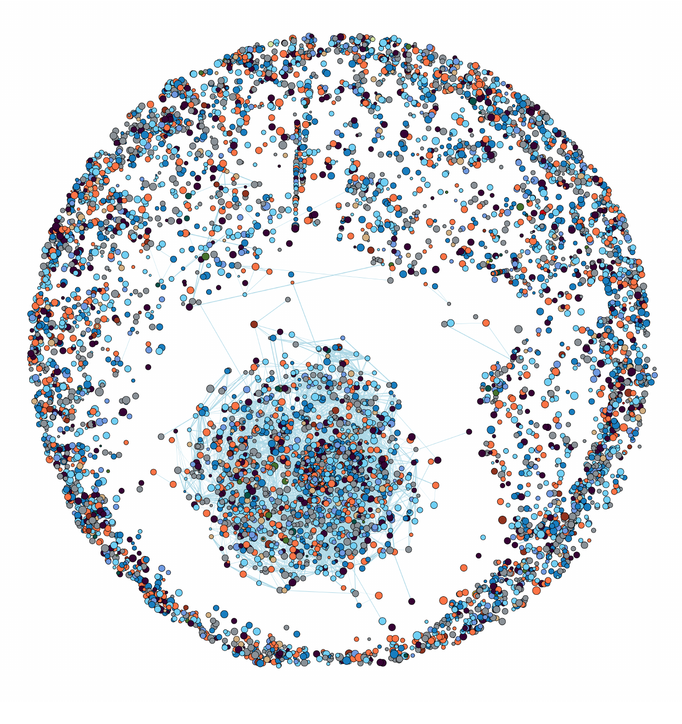
In the visualization, these ’nebulae’ will be visualized as networks. Formally,
we call these ’nebulae’ formed on the basis of ’nebula_index’ data as
Child-Nebulae. In comparison, when we put all the ‘features’ together to form a
large network, then this ’nebula’ is called Parent-Nebulae.
<<< Quick start >>>